Finding patterns of shallow organization
or
The application of a trained machine learning model by means of an example
This is a very specific analysis and probably need to be adapted vastly for other machine learning applications.
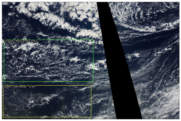
During an effort of the atmospheric department at MPI and LMD, patterns/forms of organization of shallow convection were labeled in 10.000 satellite images (https://arxiv.org/abs/1906.01906). These labels have been used to train a machine learning model to identify these patterns autonomously. In the following, the application of this trained model is shown.
Step-by-step
1. Login to mistral
ssh -L <port>:localhost:<port> user_name@mistral.dkrz.de
Choose a port for forwarding, like 8888 and use the same throughout this tutorial.
2. Allocate GPU node see also https://www.dkrz.de/up/services/analysis/visualization/visualization-on-mistral
salloc -N 1 -n 6 --mem=128000 -p gpu -A <project> -t10:00:00 -- /bin/bash -c 'ssh -L <port>:localhost:<port> -X $SLURM_JOB_NODELIST'
After the allocation of the GPU your prompt should indicate that you are now on an GPU node, like mg101.
3. Activate the appropriate conda environment
source activate environment_with_keras_installed
4. Open jupyter lab to interactively run the following commands on the GPU node.
jupyter-lab --port=<port> --no-browser
5. Load the necessary packages
%load_ext autoreload
%autoreload 2
%matplotlib inline

from pyclouds.imports import *
from pyclouds.helpers import *
from pyclouds.zooniverse import *
from pyclouds.plot import *
from PIL import Image
from tqdm import tqdm_notebook as tqdm
import pickle
from itertools import combinations
import imghdr

import keras_retinanet
import keras
from keras_retinanet import models
from keras_retinanet.utils.image import read_image_bgr, preprocess_image, resize_image
from keras_retinanet.utils.visualization import draw_box, draw_caption
from keras_retinanet.utils.colors import label_color

# import miscellaneous modules
import matplotlib.pyplot as plt
import cv2
import os
import numpy as np
import time
import pandas as pd
import glob

import tensorflow as tf
Most of these modules should be installed with
conda install --file requirements.txt
and the additional modules that we have written for this specific case you need to clone from github and install with:
python setup.py install
6. Configure the paths to the input images, the output images and the trained model
img_input_format = './InputImageFolder/*.png'
model_path = './exp5_resnet50_csv_20_inference.h5'
classification_file = 'Classifications.pkl'
You can download pretrained models at https://zenodo.org/record/2565146 (currently deactivated due to our Kaggle competition).
def get_session():
    config = tf.ConfigProto()
    config.gpu_options.allow_growth = True
    return tf.Session(config=config)

# use this environment flag to change which GPU to use
os.environ["CUDA_VISIBLE_DEVICES"] = "0"

# set the modified tf session as backend in keras
keras.backend.tensorflow_backend.set_session(get_session())
7. Load the machine learning model
If you download the model from https://zenodo.org/record/2565146 you need to convert it to an inference model first with
keras_retinanet/bin/convert_model.py /path/to/training/model.h5 /path/to/save/inference/model.h5
The training model is in this case the one downloaded from the archive. Please have a look at https://github.com/fizyr/keras-retinanet#converting-a-training-model-to-inference-model as well.
Otherwise, you can directly use
model = models.load_model(model_path, backbone_name='resnet50')
8. Load label to names mapping for visualization purposes
labels_to_names = {i: l for i, l in enumerate(['Flower', 'Fish', 'Gravel', 'Sugar'])}
9. Load the file listing
files = sorted(glob.glob(img_input_format))

** 10.Define main function**
that loads the image, applies the algorithm and returns for each identified cloud pattern a score together with the bounding box.

<code python>
def get_retinanet_preds(model, fn, thresh=0.3, min_side=800, max_side=1050):
    image = read_image_bgr(fn)
    image = preprocess_image(image)
    image, scale = resize_image(image, min_side, max_side)
    boxes, scores, labels = [o[0] for o in model.predict_on_batch(np.expand_dims(image, axis=0))]
    boxes /= scale
    boxes = boxes[scores > thresh]
    boxes = [xy2wh(*b) for b in boxes]
    labels = labels[scores > thresh]
    labels = [labels_to_names[i] for i in labels]
    scores = scores[scores > thresh]
    return np.array(boxes), labels, scores
11. Create function for visualization purposes only
def plot_img_from_fn_and_boxes(fn, boxes, labels, scores, figsize=(18, 15), show_labels=True):
    fig, ax = plt.subplots(1, 1, figsize=figsize)
    img = Image.open(fn)
    ax.imshow(img)
    ax.set_xticks([])
    ax.set_yticks([])
    for i in range(boxes.shape[0]):
        rect = patches.Rectangle((boxes[i, 0], boxes[i, 1]), boxes[i, 2], boxes[i, 3],
                                 facecolor='none',
                                 edgecolor=np.array(l2c[labels[i]]) / 255, lw=2)
        ax.add_patch(rect)
        if show_labels:
            s = labels[i] + ' - Retinanet - ' + str(scores[i])[:4]
            txt = ax.text(boxes[i, 0], boxes[i, 1], s, color='white', fontsize=15, va='top')
            txt.set_path_effects([PathEffects.withStroke(linewidth=5, foreground='k')])
    return fig

def plot_retinanet(model, fn, thresh=0.5):
    boxes, labels, scores = get_retinanet_preds(model, fn, thresh)
    fig=plot_img_from_fn_and_boxes(fn, boxes, labels, scores)
    return fig
12. Apply algorithm on your first image
fig=plot_retinanet(model, files[0], 0.4)
The result hopefully looks similar to:

This is of course only one image and can easily be applied to further images
result_dict ={}
c = 0
for file in tqdm(files[:]):
    boxes, labels, score = get_retinanet_preds(model, file, thresh=0.4)
    for b,box in enumerate(boxes):
        x,y,w,h = box
        result_dict[c] = {'labels':labels[b], 'x':x, 'y':y, 'w':w, 'h':h,
                          'score':score[b],'file':file}
        c+=1
df=pd.DataFrame.from_dict(result_dict,orient='index')
df.to_pickle(classification_file)