Satellite Cloud Observations on ICDC

If you are interested in satellite observations of clouds, the data made available by Integrated Climate Data Center (ICDC) on Levante can be a great and easy to access resource. ICDC is a service provided by the Center for Earth System Research and Sustainability (CEN) which is part of the university of Hamburg. An overview of the available datasets, which cover much more variables than what is discussed here, is given on the ICDC webpage.

There are four datasets of satellite cloud observations available from ICDC. All four datasets are gridded products for which the variables are averaged over the grid cells and time steps.

Dataset Spatial Coverage Temporal Coverage Spatial Resolution Temporal Resolution
CALIPSO CloudSat Global 07/2006–02/2011 2° x 2° Monthly
CLARA-A3 Global 01/1979–11/2023 0.25° x 0.25° Monthly
MODIS Global 02/2000 (TERRA), 07/2002 (AQUA)–07/2023 1° x 1° Daily
ISCCP Global 07/1983–06/2015 1° x 1° 3-hourly

CLARA-A3 is a product based on data from the AVHRR radiometer (5 channels from 0.6 to 12 µm; infrared to visible red), that has been aboard several satellites since 1978. MODIS is an instrument similar to AVHRR with better spectral resolution (36 channels from 0.6 to 14.4 µm). MODIS is on board of two NASA satellites that launched in the early 2000s (Aqua and Terra) and are approaching the end of their life time. CALIPSO and CloudSat are two satellites sharing an orbit and carrying multiple instruments, including active instruments in the same wavelength range (radar and lidar). All of these satellites occupy sun-synchronous orbits. This means they pass the equator at a specific local time. For example MODIS data exists for the two satellites with two different overpass times (both drifting to earlier equatorial overpass at the end of their lifetime). ISCCP is different in the sense that it is a product that relies on many different satellites and instruments, including AVHRR and its successor VIIRS.

There is a vast range of variables available from the four datasets, which are listed in detail on the ICDC webpage. Here, we just provide a subset of interesting variables to spark your interest and show how to access and plot them using python on levante.

Cool variables and the datasets they are available from:

  • Cloud Fraction (All four Datasets)
  • Ice water path (CLARA-A3, ISCCP)
  • Liquid water path (CLARA-A3, ISCCP)
  • Cloud top temperature (CLARA-A3, ISCCP, MODIS)
  • Number of cloudy pixels (CALIPSO CloudSat)
  • Effective particle radius (CLARA-A3)
  • Cloud droplet number concentration (CLARA-A3)

ICDC atmosphere data is available on Levante under the following path:

/pool/data/ICDC/atmosphere

If you need the data on a different machine, you can also download it from the ICDC webpage.

Example: Condensate path

Example: Condensate path

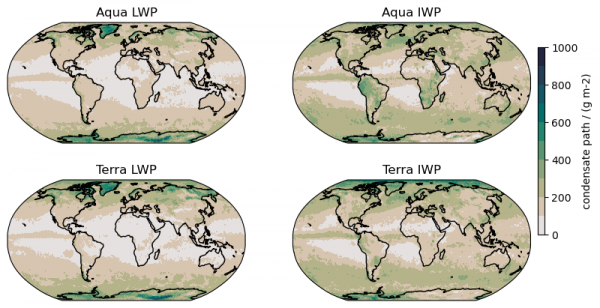
Here is an example of how to access and plot annual mean global maps of liquid water path (LWP) and ice water path (IWP) from MODIS on Levante:

   import xarray as xr
   import numpy as np
   import matplotlib.pyplot as plt
   import cartopy.crs as ccrs
   import cmocean
 
   ds_aqua = xr.open_mfdataset(
   f"/pool/data/ICDC/atmosphere/modis_aqua_cloud/DATA/2015/MODIS-C6.1__MYD08__daily__cloud-WaterPaths__2015*__UHAM-ICDC__fv0.1.nc"
   )
   ds_terra = xr.open_mfdataset(
   f"/pool/data/ICDC/atmosphere/modis_terra_cloud/DATA/2015/MODIS-C6.1__MOD08__daily__cloud-WaterPaths__2015*__UHAM-ICDC__fv0.1.nc"
   )
 
   lwp_aqua = ds_aqua.variables['cwp_liquid'].mean('time')
   lwp_terra = ds_terra.variables['cwp_liquid'].mean('time')
   iwp_aqua = ds_aqua.variables['cwp_ice'].mean('time')
   iwp_terra = ds_terra.variables['cwp_ice'].mean('time')
 
   fig, ax = plt.subplots(2, 2, subplot_kw={'projection': ccrs.Robinson()},
                        figsize=(9,5))
   lev = np.linspace(0.,1000.,11)
 
   lats = ds_aqua.variables['lat'] #same grid for Aqua and Terra
   lons = ds_aqua.variables['lon']
   llons, llats = np.meshgrid(lons, lats)
 
   cs = ax[0,0].contourf(llons, llats, lwp_aqua, lev, #vmin=lev[0], vmax=lev[-1], 
                                 transform=ccrs.PlateCarree(),cmap=cmocean.cm.rain)
   cs = ax[1,0].contourf(llons, llats, lwp_terra, lev, 
                                 transform=ccrs.PlateCarree(),cmap=cmocean.cm.rain)
   cs = ax[0,1].contourf(llons, llats, iwp_aqua, lev, 
                                 transform=ccrs.PlateCarree(),cmap=cmocean.cm.rain)
   cs = ax[1,1].contourf(llons, llats, iwp_terra, lev, 
                                 transform=ccrs.PlateCarree(),cmap=cmocean.cm.rain)
   ax[0,0].coastlines()
   ax[0,0].set_title('Aqua LWP')
   ax[1,0].coastlines()
   ax[1,0].set_title('Terra LWP')
   ax[0,1].coastlines()
   ax[0,1].set_title('Aqua IWP')
   ax[1,1].coastlines()
   ax[1,1].set_title('Terra IWP')
 
   cbar_ax = fig.add_axes([0.91, 0.3, 0.01, 0.5]) #xpos, ypos, width, height
   cbar=fig.colorbar(cs, cax=cbar_ax,orientation='vertical')
   cbar.ax.set_ylabel('condensate path / (g m-2)')
 
   plt.savefig('MODIS_condensate_path_2015.pdf')

Slightly modifying the script above with a different data path and variables names, one can look at the condensate path from CLARA-3:

   ds_clara_i = xr.open_mfdataset(
    f"/pool/data/ICDC/atmosphere/eumetsat_clara3_cloud/DATA/IceWaterPath/MONTHLY/IWPmm2015*01000000319AVPOS01GL.nc"
   )
   ds_clara_l = xr.open_mfdataset(
    f"/pool/data/ICDC/atmosphere/eumetsat_clara3_cloud/DATA/LiquidWaterPath/MONTHLY/LWPmm2015*01000000319AVPOS01GL.nc"
   )
   lwp_clara = ds_clara_l.lwp.mean('time')
   iwp_clara = ds_clara_i.iwp.mean('time')

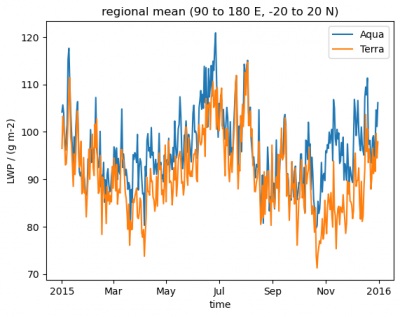
Selecting a region and looking at the time series, e.g., for the warm-pool region (assuming that grid boxes have the same size which is hopefully not too wrong around the equator):

   ds_aqua.cwp_liquid.sel(lon=slice(90,180)).sel(lat=slice(20.,-20.)).mean('lat').mean('lon').plot(label='Aqua')
   ds_terra.cwp_liquid.sel(lon=slice(90,180)).sel(lat=slice(20.,-20.)).mean('lat').mean('lon').plot(label='Terra')
   plt.legend()
   plt.title('regional mean (90 to 180 E, -20 to 20 N)')
   plt.ylabel('LWP / (g m-2)')

Example: Comparison of Cloud Area Fraction

Example: Comparison of Cloud Area Fraction

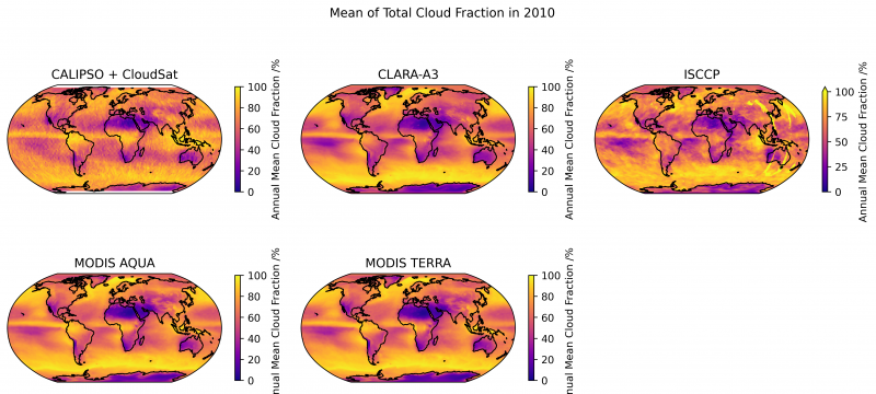
Here is an example of how to access and plot a comparison of the annual mean cloud area fraction from the ICDC datasets on Levante. The script can be downloaded and executed to produce the following plot:

cloud_area_fraction_comparison_script.py
'''The following script plots annual mean of cloud area fraction for the 4 different satellite products from ICDC for a given year. The scripts takes circa. 3 minutes to plot data and requires Python >= version 3.10 with numpy, matplotlib, xarray, netcdf4, cartopy and dask. You may also need to update your dask diagnostics, e.g. via "python -m pip install dask[diagnostics] --upgrade".'''
 
import numpy as np
import matplotlib.pyplot as plt
import xarray as xr
import cartopy.crs as ccrs
 
### --- src functions --- ###
def figure_setup(title):
  ''' returns figure with 5 axes that use the Robinson projection
  and have coastlines.'''
 
  fig = plt.figure(figsize=(12, 6))
  axs = []
  a=1
  for i in range(3):
    for j in range(2):
      axs.append(fig.add_subplot(2, 3, a, projection=ccrs.Robinson()))
      a+=1
  fig.delaxes(axs[-1])
  for ax in axs:
    ax.coastlines()
 
  fig.suptitle(title)
 
  return fig, axs[:-1]
 
def plot_annualmean_on_axis(ax, axis_title, cbar_label, dataset_path, var_name,
                            scale_factor, cmap='plasma', vmin=0, vmax=100):
  '''creates a single dataset from all the (netdcf) files found in the 'dataset_path',
  then takes the time mean of the variable called 'var_name' in the dataset, and
  multiplies it by a scale_factor. Finally plots the mean values as an image
  on the given axis 'ax' with title 'axis_title'.'''
  ds = xr.open_mfdataset(dataset_path)
 
  ntimes = ds.time.size
  print('Mean over '+str(ntimes)+' times in datasets from '+dataset_path)
  yearmean = ds[var_name].mean('time') * scale_factor
 
  cbar_kwargs={'shrink': 0.5, 'label': cbar_label}
  yearmean.plot(ax=ax, transform=ccrs.PlateCarree(), cmap=cmap,
                cbar_kwargs=cbar_kwargs, vmin=vmin, vmax=vmax)
  ax.set_title(axis_title)
 
def save_figure(fig, savefig_name='figure1.png', is_show=True):
  ''' saves 'fig' as file called 'savefig_name'.'''
 
  fig.savefig(savefig_name, dpi=400, bbox_inches="tight", facecolor='w', format="png")
  print("Figure saved as: "+savefig_name)
 
  if is_show:
    plt.show()
### --------------------- ###
 
### --- input parameters --- ###
year = '2010' # year to plot (must be available in all 5 products)
fig_title = 'Mean of Total Cloud Fraction in '+year
cbar_label = 'Annual Mean Cloud Fraction /%'
savefig_name = "./cloud_area_fraction.png"
 
icdcpath = '/pool/data/ICDC/atmosphere/'
basepaths = { # base of paths to netcdf files to use in plotting of each satellite product
  'calipso_cloudsat': icdcpath+'calipso_cloudsat_cloudcover/DATA/',
  'clara3': icdcpath+'eumetsat_clara3_cloud/DATA/',
  'isccp': icdcpath+'isccp/DATA/',
  'modis_aqua': icdcpath+'modis_aqua_cloud/DATA/',
  'modis_terra': icdcpath+'modis_terra_cloud/DATA/',
}
 
datasets = { # full paths to netcdf files to use in plotting of each satellite product
    'calipso_cloudsat': basepaths['calipso_cloudsat']+'UCAR__merged_cloudsat-calipso_totalcloudcover__UCAM-ICDC__v0.1__2deg__'+year+'*.nc',
    'clara3': basepaths['clara3']+'FractionalCloudCover/global/MONTHLY/CFCmm'+year+f'*01000000319AVPOS01GL.nc',
    'isccp': basepaths['isccp']+'hgg/'+year+'*/ISCCP-Basic.HGG.v01r00.GLOBAL.'+year+'.*.01.*.GPC.10KM.CS00.EA1.00.nc', 
    'modis_aqua': basepaths['modis_aqua']+year+'/MODIS-C6.1__MYD08__daily__cloud-Fractions__'+year+'*__UHAM-ICDC__fv0.1.nc',
    'modis_terra': basepaths['modis_terra']+year+'/MODIS-C6.1__MOD08__daily__cloud-Fractions__'+year+'*__UHAM-ICDC__fv0.1.nc',
  }
 
dataset_names = { # names of each satellite product
  'calipso_cloudsat': 'CALIPSO + CloudSat',
  'clara3': 'CLARA-A3',
  'isccp': 'ISCCP',
  'modis_aqua': 'MODIS AQUA',
  'modis_terra': 'MODIS TERRA',
}
 
variable_names = { # names of cloud area fraction in each satellite product
  'calipso_cloudsat': 'cf',
  'clara3': 'cfc',
  'isccp': 'cldamt',
  'modis_aqua': 'cfrac',
  'modis_terra': 'cfrac',
}
 
variable_scalefactor = { # multiply variable by scale_factor for each satellite to convert to %
  'calipso_cloudsat': 100,
  'clara3': 1,
  'isccp': 1,
  'modis_aqua': 100,
  'modis_terra': 100,
}
### ------------------------ ###
 
### --- plotting of data --- ###
datasets2plt = ['calipso_cloudsat', 'clara3', 'isccp', 'modis_aqua', 'modis_terra']
fig, axs = figure_setup(fig_title)
for ax, d in zip(axs, dataset_names.keys()):
  plot_annualmean_on_axis(ax, dataset_names[d], cbar_label, datasets[d],
                          variable_names[d], variable_scalefactor[d])  
fig.tight_layout()
save_figure(savefig_name)
### ------------------------ ###


ICDC gathers data from many different sources (see Datasets from ICDC) and thus it is not possible to thoroughly address their respective biases and shortcomings here. All satellites observe the atmosphere from above and most instruments we use are passive sensors. Earths outgoing radiation is measured at discreet wavelength bands and this information is used to deduct the properties of the source of this radiation. For some wavelengths bands there is a good direct correlation to properties in earths atmosphere or surface. Satellite products try to combine information on different bands to make this correlation more robust. Still, biases remain. The following discusses cloud cover and condensate paths exemplary.

Cloud cover

Satellite cloud cover estimates usually work by having an expectation on how the ground should look like and then setting a threshold on how much the actual value is allowed to differ. This clearly depends on the actual threshold. More importantly it depends on the expected ground properties and how much they differ from the clouds properties. Cloud cover products tend to be more precise over ocean than over land because the contrast in the visible is usually stronger, they work better with high clouds than with low clouds because the contrast in thermal radiation is stronger and they have problems with ice covered land surface for both of the above reasons. False positives in cloud cover over high albedo land surfaces also have implications for products that use that cloud mask (e.g. land surface temperature; Wislon et al., 2014 ). There are concerns that satellite derived cloud cover is systematically overestimated ( Schuetz, 2007).

Condensate path

Uncertainties deriving from unknown surface contributions can hinder satellite based measurements of condensate paths (like they do for cloud cover products). How much the surface contributes to the signal also depends on the analysed wavelength. Microwave measurements penetrate the atmosphere easily and thus higher surface contributions. This makes them have high uncertainties over highly variable land surfaces and thus they are usually available over ocean only. Infrared based measurements on the other hand penetrate less. This makes them less susceptible to surface contributions, but they saturate easily if the cloud is too thick, making the lower levels invisible to the satellite instrument.

In general infrared based liquid water path measurements are considered to perform better than microwave based measurements (Stengel et al., 2015), but they have a zonal bias that is strongly correlated with the solar zenith angle. This bias can be greater than a factor of 2 in global and zonal averages of LWP. This makes it challenging to use for comparison to model data (Khanal et al., 2020 and references therein).

Using data provided by ICDC is great, but the available data is limited. The four datasets that are available for satellite cloud observations are all high-level gridded products. This is good if you are interested in climatological values, however, if you are looking for instantaneous values you won't find them on ICDC.

If you are interested in lower level, non-gridded versions of the datasets provided by ICDC, you can either get lucky and find that some working group already saved it to Levante, or you have to download it from the NASA or EUMETSAT webpages. The working group of Stefan Buehler maintains some CALIPSO CloudSat data and the python package Typhon which offers the functionality to read it.